Being able to rapidly benchmark and predict shelf stability without waiting months is crucial for formulators wanting to fast-track products to market. At the Centre for Industrial Rheology, we exploit three critical analytical techniques that combine to deliver powerful predictive contributions to the stability of emulsions and suspensions.

By leveraging the combined capabilities of Dynamic Light Scattering and Zeta Potential, Bulk Rheology, and Interfacial Rheology, we can comprehensively map metrics associated with stability.
| Metric | What it measures | Relevance to Stability | Temperature Range (°C) |
|---|---|---|---|
| Zeta Potential (mV) | Electrostatic repulsion between particles | Quantifies the electrostatic repulsion around a particle, which contributes to preventing aggregation. Identifying the isoelectric point allows for pH optimisation. | 0 to 120 |
| Zero Shear Viscosity (cP, Pa·s) | Viscosity at close to at-rest conditions. | Represents the material’s resistance to flow at rest, with higher values correlating with the ability to immobilise droplets or particles, resisting sedimentation or creaming. | -45 to 500 |
| Yield Stress & Structure | Complex Modulus (Pa) and Phase Angle (°) | The stress required to make a material flow. It can be seen as the “strength” of the internal network when the product is sitting still. A sufficient yield stress acts as a physical net that immobilises particles or droplets. | -45 to 500 |
| Oscillatory Frequency Sweeps | Storage and Loss Modulus (Pa) | Time-dependent viscoelastic behaviour. We look for a loss of elastic dominance at low frequencies, indicating that over long periods, the structure will relax and flow like a liquid. | -45 to 500 |
| Thixotropic Rates (Pa) | Breakdown and recovery before and after shear | Determines how quickly the structure recovers after the application and cessation of shear. | -45 to 500 |
| Interfacial Rheology (mN/m) | Rigidity of interfaces | Influences the creation and stabilisation of interfaces, which is extremely important for emulsions and even foams. | 20 to 60 |
By utilising these methods, we can analyse your products under a wide range of processing and storage conditions. With all our instruments, we have temperature control capabilities and thus can provide insights into thermal stability, on top of a holistic view of your product’s long-term behaviour.
Book a chat with our team to discuss how these techniques can be used to characterise your products
Contact Us
This article goes into these techniques in more detail and explains how they are relevant to probing stability.
Electrostatic Stabilisation Strategies – Zeta Potential

To measure zeta potential, we utilise the Malvern Zetasizer Ultra Red, the top-of-the-range instrument for this analysis. This parameter is measured using electrophoretic light scattering, where an electric field is applied to the sample, causing charged particles to move. By measuring the velocity of this movement, the instrument calculates the zeta potential.
Understanding the Charge Structure
Every particle in a suspension or droplet in an emulsion develops a surface charge. The environment surrounding the particle is visualised in the concept of the electrical double layer:
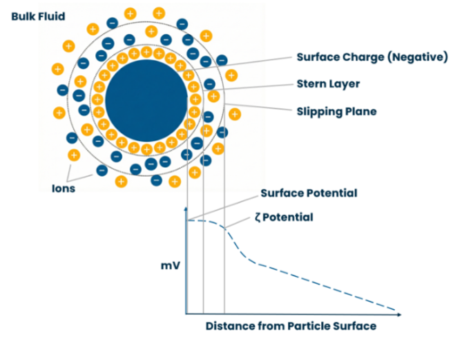
- Stern Layer – A layer of ions oppositely charged to the particle, bound tightly to the surface.
- Diffuse Layer – A secondary layer of ions that are loosely associated, forming a cloud around the particle.
Within the diffuse layer, a theoretical boundary exists, known as the Slipping Plane. Zeta potential is the electrical potential measured specifically at this slipping plane.
Interpreting the Data
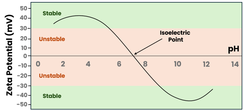
The magnitude of the zeta potential gives us a direct indication of the repulsive forces around a particle.
- > 30 mV (Stable) – Generally, a zeta potential with a magnitude greater than 30 mV, either positive or negative, indicates good stability. The electrostatic charge is sufficient to repel neighbouring particles, preventing them from approaching close enough to aggregate.
- < 30 mV (Unstable) – When the magnitude drops below 30 mV, the repulsive barrier is weak. Over time, Brownian motion will lead to collisions, resulting in flocculation or coalescence.
The Isoelectric Point
Zeta Potential is often heavily influenced by the pH of the continuous phase. As such, Zeta Potential testing is very commonly used to determine the isoelectric point. This is the specific pH value at which Zeta Potential is 0 mV. At this point, the system possesses no net charge to provide repulsion, placing it in its most unstable state.
By performing a pH titration, we map the zeta potential across a wide pH range. This highlights the danger zones for your formulation. If your product is formulated near its isoelectric point, you are fighting a losing battle against thermodynamics. Our testing identifies this risk early, providing the data needed to adjust the pH or formulation to ensure a stable product.
Physical Stabilisation Strategies – Rheology
Zero-Shear Viscosity
The zero-shear viscosity reflects the viscosity of a product when it is effectively at rest. It is arguably one of the most practical indicators of stability, yet it is frequently overlooked as viscometers lack the torque sensitivity to perform such tests.
Our research rheometers in the lab offer extraordinary sensitivity, detecting low stresses that extend far beyond the range of typical viscometers. They are capable of detecting rotational speeds as slow as 1 revolution every 3 months. Despite this, we obtain rapid results in as little as 30 minutes. Examples of outputs from this test are shown below.
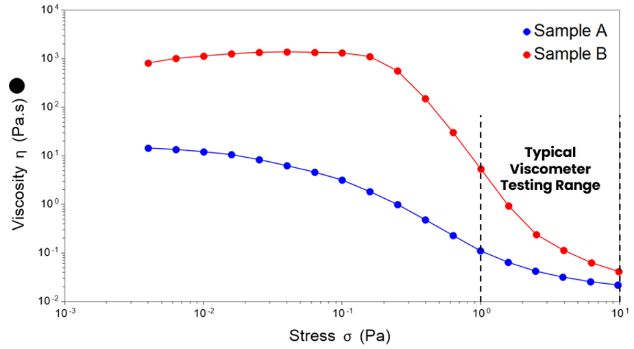
A high zero-shear viscosity in the external phase is desirable as it helps to immobilise particles and droplets. A high zero-shear viscosity of the entire system is also a valuable diagnostic, as it can predict long-term stability; however, it can also be an indicator that aggregation or flocculation has occurred.
The plateau observed at low stresses reflects the zero-shear viscosity. Figure 5 shows that both products’ zero shear viscosities sit well above the lowest-stress data obtainable through a typical viscometer. A difference of over a decade is observed for sample A, and a huge difference of over 3 decades is observed for sample B.
Breakdown and Recovery – Thixotropy
Thixotropy describes the time-dependent change in viscosity following either the application or cessation of shearing. In suspensions and emulsions, the breakdown and recovery of colloidal structures is typically time-dependent rather than instantaneous, requiring time to reach a new equilibrium. Understanding this time-dependence is crucial for predicting how a product may behave following the transition from a high-shear to a low-shear state.
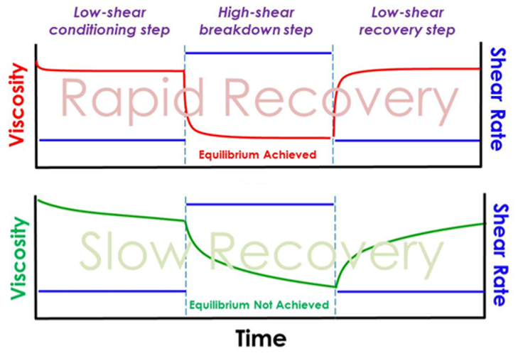
The thixotropic breakdown or recovery rate is a commonly used output of a thixotropy measurement. By probing both the breakdown and recovery of structure, we gain a holistic view of suspension or emulsion behaviour.
Yield Stress & Structure
To get further insights into stability, we go beyond viscosity to look at viscoelasticity and the concept of yield stress. Yield stress is the minimum amount of stress required to make a material flow. Think of it as the “strength” of the internal network when the product is sitting still. A sufficient yield stress acts as a physical net that immobilises particles or droplets. If the yield stress is strong enough to counteract the gravitational force exerted by the dispersed particles, sedimentation and creaming are effectively inhibited, aiding long-term shelf stability.
To measure this, we employ oscillatory techniques, where we gently “wobble” the sample to allow us to probe the delicate internal structure present without destroying it. The complex modulus is obtained through these techniques, which describes the overall resistance to deformation, essentially, the rigidity of the sample. A higher complex modulus indicates a stiffer, more robust network. The phase angle is also obtained, which describes the relative contributions between elastic and viscous behaviour. A phase angle of 0° indicates elastic dominance, where the material behaves more like a solid. A phase angle of 90° indicates viscous dominance, where the material behaves like a liquid.
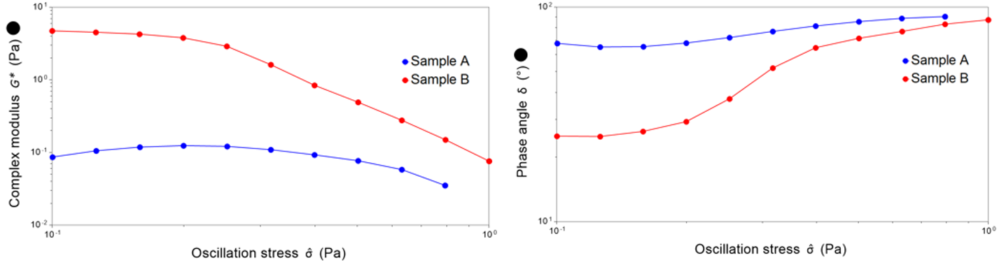
For these emulsions, sample A displays a yield stress of 0.31 Pa. In contrast, sample B exhibits a phase angle exceeding 45° even at the lowest stresses. This is indicative of a very delicate structure, with yield stress becoming an irrelevant metric in this situation. The data in this case indicates that sample A may be significantly more stable than sample B on the shelf.
Time-dependent Viscoelastic Behaviour
Some materials may appear to be stable during quick handling yet prove unstable over long periods. To understand this, we investigate time-dependent viscoelastic behaviour by oscillating a sample across a wide range of frequencies while maintaining a constant stress.
The complex modulus can then be split out into its in-phase and out-of-phase responses. Storage modulus reflects the elastic (solid-like) response, whereas loss modulus reflects the viscous (liquid-like) response.
With these tests, we are essentially identifying the potential “relaxability” of the network by looking specifically for a loss of elastic dominance at low frequencies. If a material becomes more viscous at low frequencies, it indicates that over longer timescales, the structure will relax and flow more like a liquid, leading to instability.
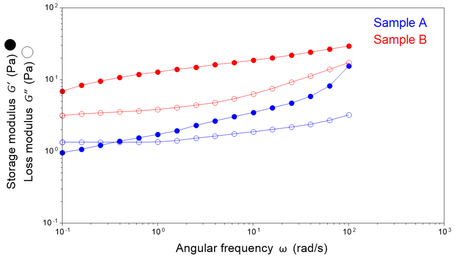
Sample A maintains elastic dominance across the entire frequency range tested, indicating robust stability. Conversely, sample B exhibits a loss of elastic dominance at low frequencies, a characteristic indicator of instability.
Interfacial Rheology
While bulk rheology examines the liquid as a whole, interfacial rheology focuses specifically on the liquid-air or liquid-liquid interface. This interface plays an important role in resisting coalescence.
We capture the dynamics of this interface using oscillatory dilatational techniques. This is where we oscillate a droplet to expand and contract its surface area. This allows us to measure how surface-active molecules, such as protein emulsifiers, migrate to and from the interface, providing insights into the viscoelasticity of that boundary. This is a key metric for stability, as a rigid and elastic interface acts as a protective barrier that tends to suppress the coalescence of emulsified droplets, effectively preventing them from merging and separating over time.
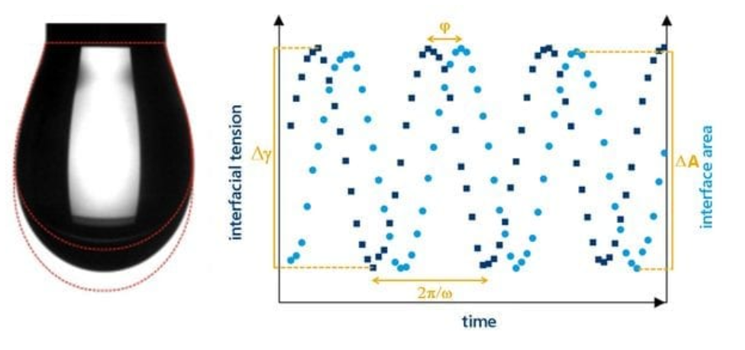
Interfacial tension and interfacial rheology are of great interest to formulators due to their influence in creating and stabilising interfaces, such as in emulsions or even foams.
Contact us to explore how we can probe stability for your suspension or emulsion

Related Articles;
Zero Shear Viscosity for Emulsion and Suspension Stability
Emulsion Stability: Strong and Stable or Weak and Feeble
Wasif Altaf serves as an Applications Specialist at the Centre for Industrial Rheology, leveraging a chemical engineering background (BEng) to bridge theory and practice. His work focuses on advanced rheological characterisation.