
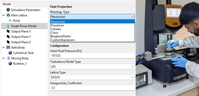
There is perhaps no greater risk in computational fluid dynamics than spending hours on simulations, quietly unaware of the inadequacy of your rheology data. Ultimately, your simulation is only as good as the data you feed it. Whether you are using Ansys Fluent, Star-CCM+, SimScale, COMSOL, M-Star, or Autodesk, you may have asked, where can you get reliable material constants for your sample from?
Relying on estimated data or generic library values can lead to inaccurate simulations. In the context of complex fluid flow, this is more than just a margin of error. Incorrect yield stress values can generate fake dead zones, while inaccurate zero-shear viscosity can result in meaningless mixing power calculations. In practice, this can lead to incorrect design decisions or costly late-stage corrections.
At the Centre for Industrial Rheology, we specialise in bridging the gap between a physical sample and a simulation-ready data set. Our focus is on providing modelling-ready rheology data, and we are well-equipped to gather this data accurately and quickly.
To ensure the full definition of fluid properties required by solvers, we provide comprehensive rheology, viscosity, and density measurements across a wide range of temperatures. We also understand that every solver is different; whether your workflow requires specific units of Pa·s or cP, we deliver data in solver-ready units and formats tailored to your needs.
Contact our lab to discuss your analysis needs
The Models We Support – From Lab to Solver Input
In addition to generating data, we can advise on which specific mathematical model may be best suited for your sample. Below are some common non-Newtonian models we provide data for, along with the specific metrics we can extract from your samples.
Key Symbols:
Shear Stress (τ)
Shear Rate (γ̇ )
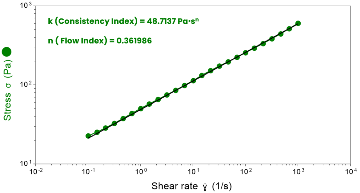
Power Law Model
The power law model is commonly used for non-Newtonian fluids. We provide the coefficients needed to describe how viscosity changes with shear rate.
τ = k · γ̇ n
We deliver:
- Consistency index (k) – Quantifies the fluid’s viscosity at a shear rate of 1s-1.
- Flow Index (n) – quantifies the degree of shear-thinning behaviour.
- n < 1 (Pseudoplastic / Shear-thinning): The most common non-Newtonian behaviour, where viscosity decreases as the shear rate increases.
- n = 1 (Newtonian): Viscosity remains constant regardless of the shear rate applied.
- n > 1 (Dilatant / Shear-thickening): Viscosity increases as the shear rate increases.
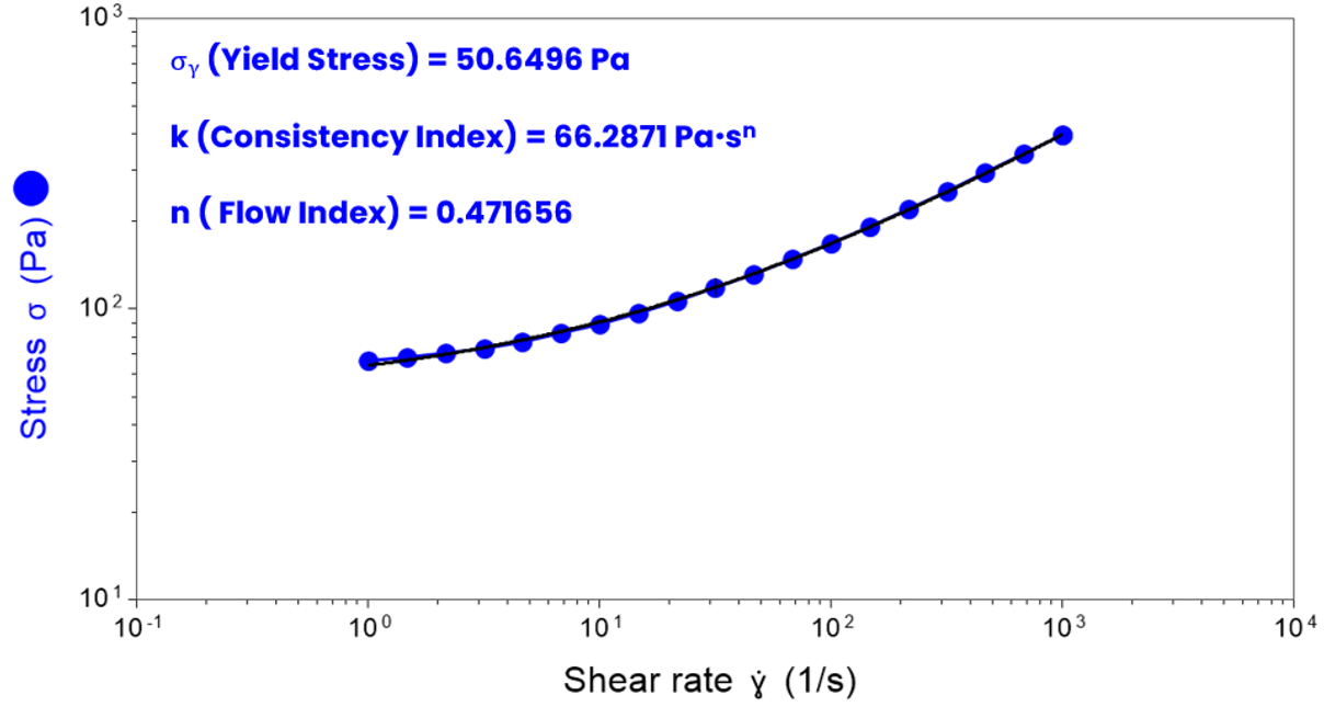
Herschel-Bulkley Model
This model is used for ‘yield-stress’ fluids such as pastes, gels, and slurries that require an applied stress before they begin to flow. This is essentially a power law model with an added quantification for yield stress. In this model, the yield stress is defined by extrapolating the shear stress back to a shear rate of zero.
If you are familiar with this model, you may have encountered numerical instability in CFD simulations due to the sharp transition at the yield point. To assist with this, we can advise on regularisation parameters such as the Papanastasiou model, which introduces a smoothing parameter that allows for a continuous mathematical transition between the solid-like and fluid-like states.
τ = σy + k · γ̇ n
We deliver:
- Yield Stress (σy) – the stress required to make a material flow
- k and n values – describing the flow behaviour once the yield point is exceeded
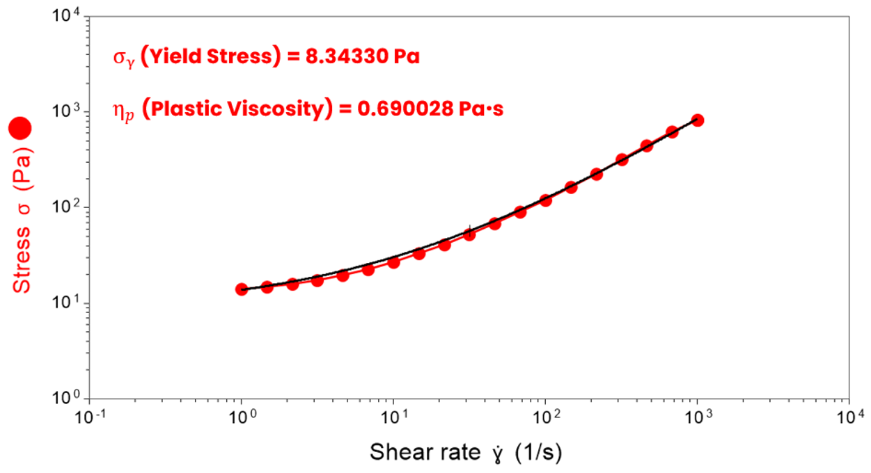
Bingham and Casson Models
These models are utilised for materials exhibiting “plastic” behaviour. They describe a material that stays rigid until the yield stress is reached, after which it flows with a constant (Bingham) or evolving (Casson) plastic viscosity.
τ = σy + ηp · γ̇
√τ = √σy + √ηp·γ̇
We deliver:
- Yield Stress (σy) – the stress required to make a material flow
- Plastic Viscosity (ηp) – the slope of the stress curve in the high-shear region
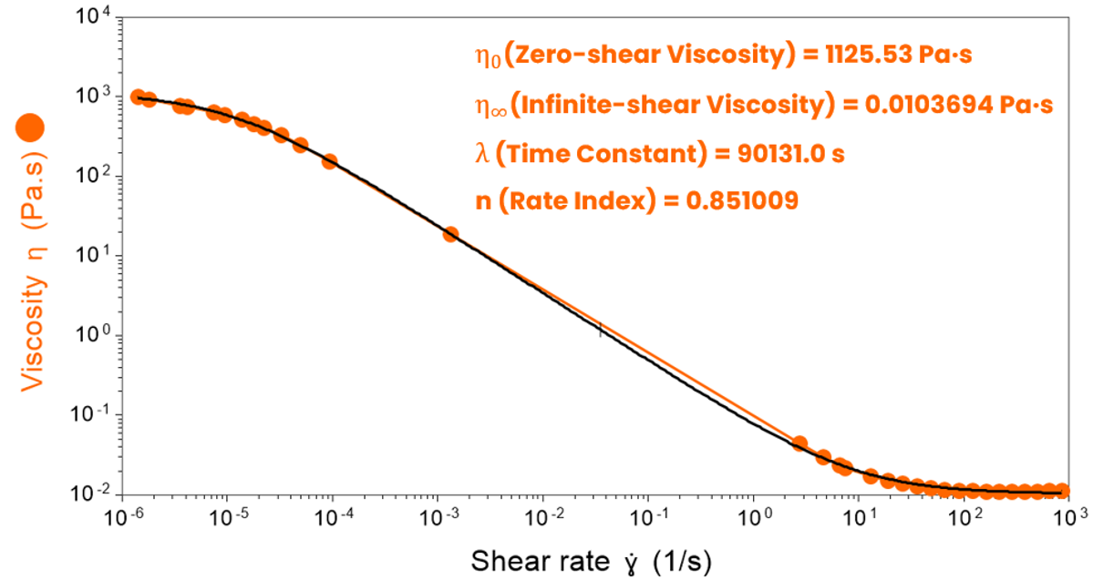
Cross and Carreau-Yasuda Models
When your simulation requires a complete profile, these models are the gold standard. They capture the zero-shear plateau, the shear-thinning transition, and the infinite-shear plateau.
η = η∞ + (η0 − η∞) / [1 + (λ·γ̇)n]
η = η∞ + (η0 − η∞)[1 + (λ·γ̇ )a](n−1)/a
We deliver:
- Zero Shear Viscosity (η0) – the maximum plateau viscosity of the fluid when it is effectively at rest
- Infinite Shear Viscosity (η∞) – the minimum plateau viscosity at high shear rates
- Time Constant (λ) – characterises the onset of shear-thinning
- Flow Index (n) – quantifies the intensity of shear-thinning
Summary – Your Partner in CFD Data
Whether you are modelling flow through a heat exchanger, a pump, or even blood pumping within the chambers of the heart, we have spent decades working with a variety of material types. We handle all the complexities with rheological characterisation so you can focus on the simulation. With a suite of specialised accessories, we can characterise even the most difficult samples accurately, providing you with a complete, solver-ready data set.
Contact us today for a chat about your project, and let’s get your simulation moving with data you can trust.

Related Articles:
Predicting Formulation Stability: Advanced Insights for Suspensions and Emulsions
Wasif Altaf serves as an Applications Specialist at the Centre for Industrial Rheology, leveraging a chemical engineering background (BEng) to bridge theory and practice. His work focuses on advanced rheological characterisation.